

Conventional gene expression analysis
= Analysis of cell populations together
➔ You can see the overall average.

scRNA-Seq
= Analysis of individual cells
➔ We can tell the difference between individual cells.
This method examines the gene expression of individual cells that make up a tissue.
Bulk RNA-Seq detects average gene expression in a cell population, whereas single cell RNA-seq analysis (scRNA-seq), which examines gene expression in individual cells, allows detailed analysis of the function and activation state of the various cells that make up a tissue. The scRNA-seq analysis is a method to analyze the function and activation state of various cells constituting a tissue.
・
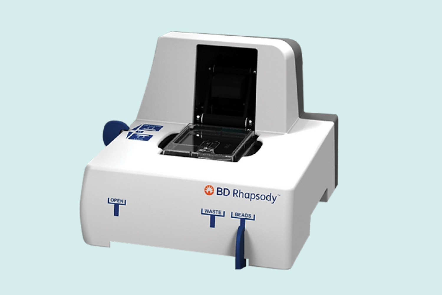
This is whole transcriptome scRNA-seq analysis using nanowells and magnetic beads on the BD Rhapsody system.
*Certified by Becton Dickinson Japan K.K. as a service provider using the BD Rhapsody™ Single Cell Analysis System
・
Our proprietary total cDNA amplification method from solid-phase beads (TAS-Seq method) realizes highly sensitive and accurate analysis.
・
Multiplex analysis is supported, allowing analysis of multiple samples without much cost. (The USB method allows labeling of any cell type or organism. Please refer to the Multiplex section in the "Technology " section.)
・
Simultaneous measurement of mRNA and cell surface protein expression (CITE-seq: Cellular Indexing of Transcriptomes and Epitopes by sequencing) is also available. Please contact us from the "Contact Us" page.
・
Multiplex analysis using BD's SampleTag, BioLegend's Hashtag, etc. is supported, allowing analysis of multiple samples without much cost.
・
BD Rhapsody Express systems can be rented and workers can be dispatched to the site (at an additional cost).
・
We have experience analyzing leukocytes derived from mouse lung, pancreatic la islet, kidney, human lung and gastric cancer biopsy samples, and human peripheral blood neutrophils.
・
Click here to see the analysis use paper .
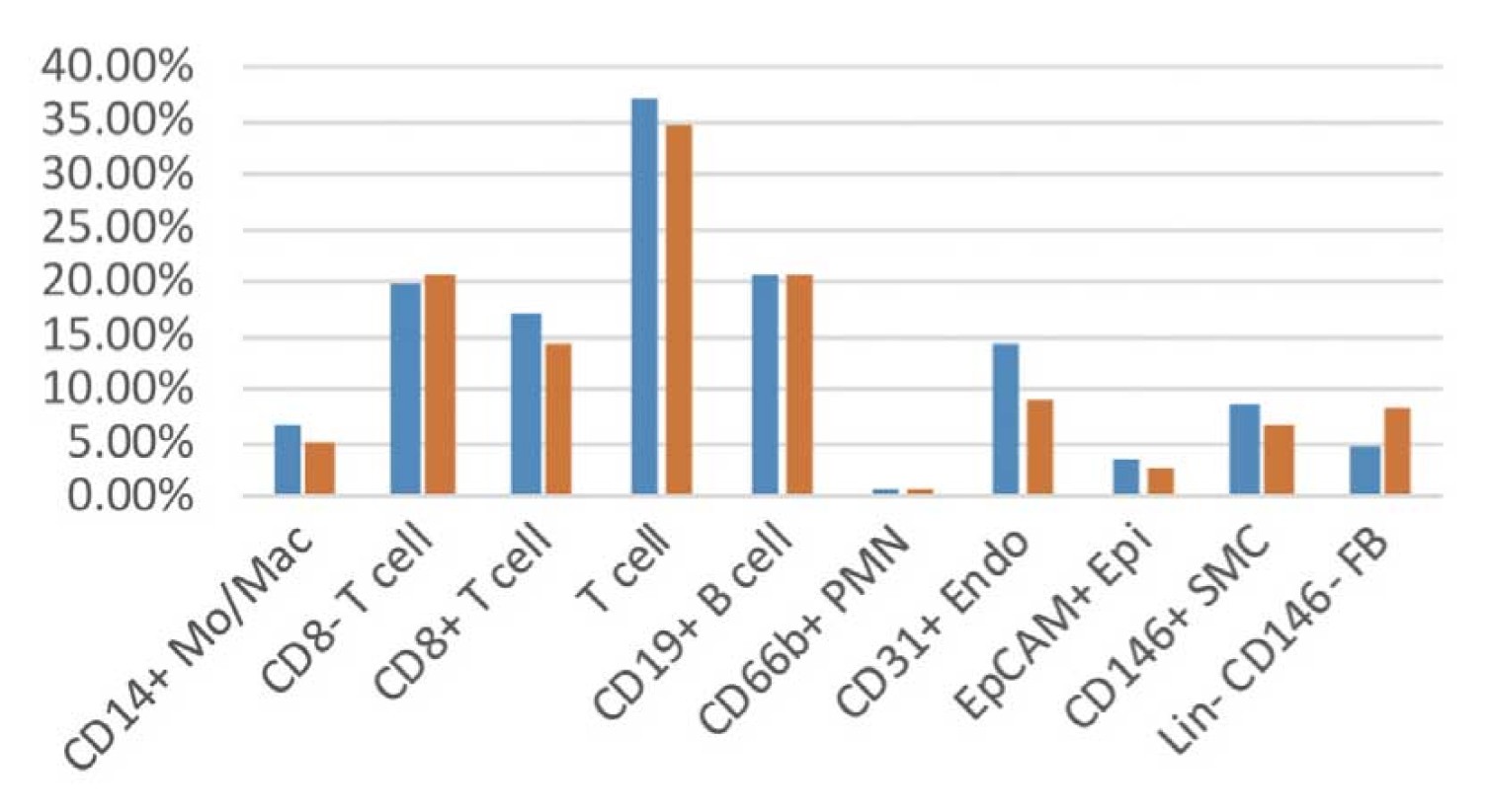
Example of analysis of human rheumatic lung
S1:4055 cells and S2:4938 cells were pooled, clustered on PCA space, and the results were visualized by dimensional compression using tSNE.
The combination of ImmunoGeneTeqs Rhapsody and TAS-Seq method has almost no batch effect and basically does not require batch effect correction.
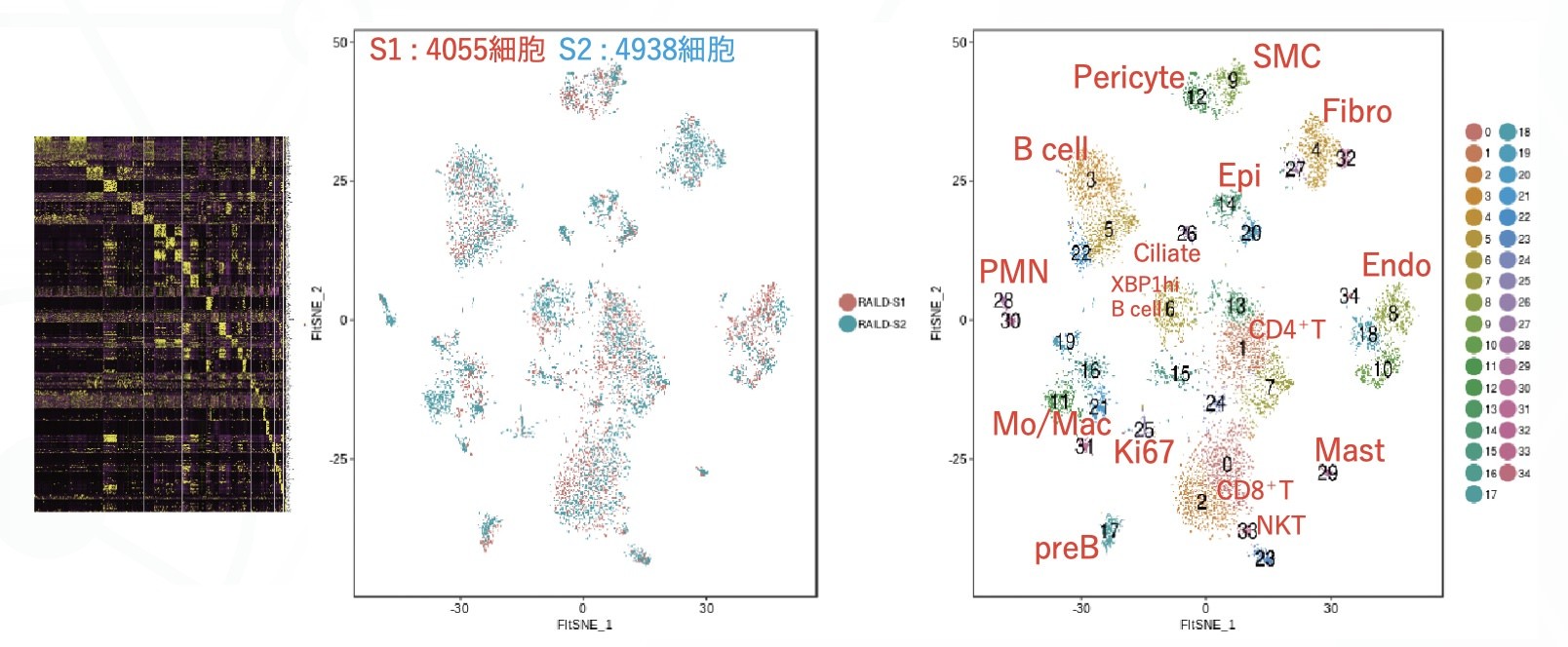
* Clustering refers to finding cells with similar gene expression patterns and dividing them into clusters (populations).
* In the case of data measured in different experimental environments (batches), there is a "batch effect" (inter-experimental error) that causes differences in data between batches, even for the same organ or cell. Batch effect correction may be necessary when these effects make data interpretation difficult, such as when interpreting clustering results. Batch effect correction may mask biological differences.
Comparison of cell detection accuracy between flow cytometers and various techniques in mouse lung cells
Compared to flow cytometer data, TAS-seq correlates well with flow cytometers and provides accurate cell composition data.
10X v2 data from other methods over-detected macrophages and under-detected fibroblast fractions. (See red box)
Smart-seq2 data over-detected endothelial cells and monocytes and lost alveolar macrophages (see green box).
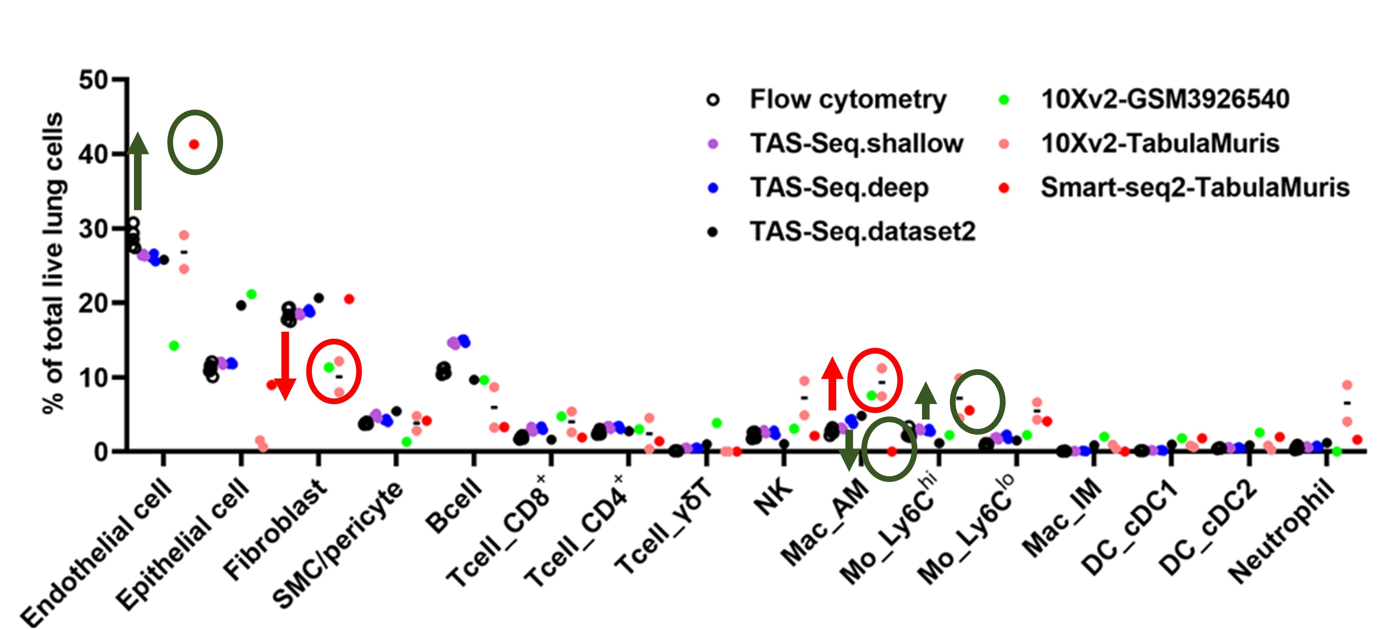


Shichino S. et al. Communications Biology volume 5, Article number: 602 (2022)
Detection of intercellular communication in mouse lung


Development of TAS-seq2
We have optimized the reaction system of TAS-Seq and developed TAS-Seq2 with even higher detection sensitivity.


Example of nuclear analysis of cells derived from mouse liver specimen using TAS-Seq2

*10X nuclear conditioning kit with anti-nuclear pore complex hashtags approx. 20000-30000 reads / nucleus
TAS-Seq2 enables more sensitive detection of genes in cell nuclei than other methods

10X v3.1: Published mouse liver sample data (SRX14774301, SRX14774300)
Samples with analysis results
single-cell RNA-seq
Mouse
etc.
Human
etc.
Cultured Cell
etc.
Other Species
etc.
single-nucleus RNA-seq
Mouse
etc.
We send necessary equipment and reagents to you.
➊ Cell loading
(Spontaneous drop, Poisson distribution)
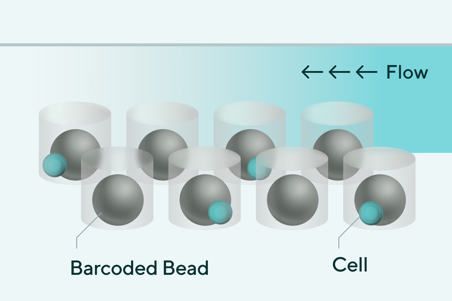
➋ Loading of excessive amounts of beads
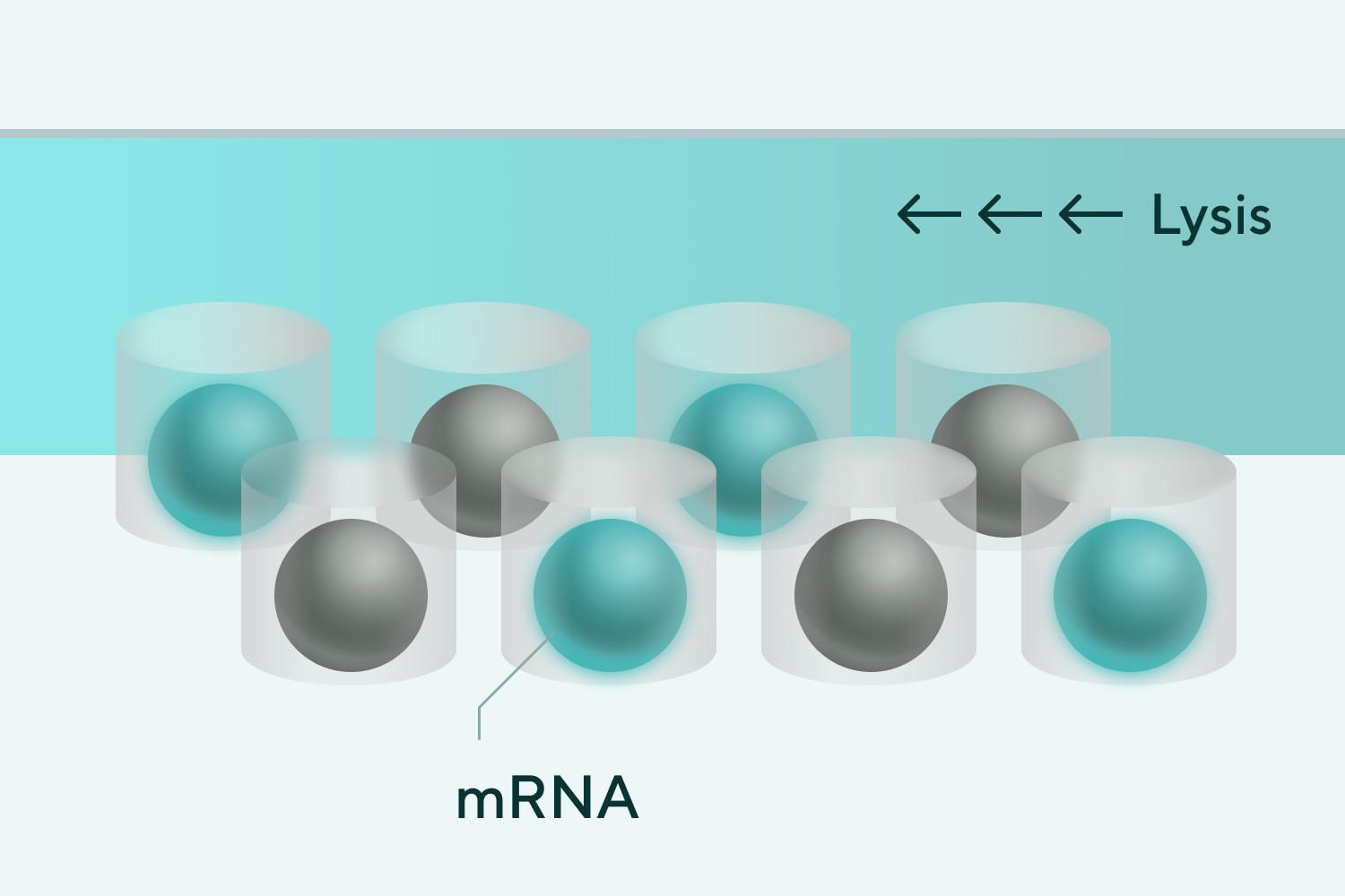
➌ Cell solution, various cell-derived mRNAs supplemented with beads
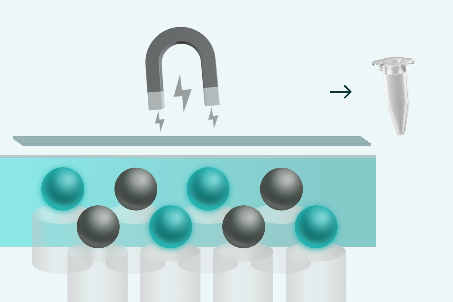
➍ Bead recovery and reverse transcription
Customer sends us samples that have been ➊~➍ done onsite.
Matters to be checked in advance
* For multiplex analysis, please refer to the FAQ page "About Multiplex Analysis".
How to request
Sample acceptance
・
cDNA synthesized by our specified protocol (IGT will undertake cDNA amplification and subsequent steps)
・
Frozen cells (IGT is contracted to perform cell antibody staining and cDNA synthesis and beyond)
・
Frozen tissue (IGT is entrusted with the preparation of cell suspensions from tissue and beyond)
* Please contact us if you wish to make adjustments from frozen cells or tissues.
* When cryopreserving cells and tissues, please use the preservation solution and freezing method specified by us.
How to send samples
・
Please make sure that the sample is dry and leak-free, and send it to the shipping address below. (Available until 5:00 p.m. on weekdays)
・
When shipping BD Rhapsody beads that have been reverse-transcribed using our specified protocol, please ship refrigerated.
・
When shipping frozen cells/tissues, please include enough dry ice to maintain the frozen state and send via frozen delivery.
* Please send by next day except for remote areas.
Send samples to
〒277-0882
千葉県柏市柏の葉6丁目6番2号
三井リンクラボ柏の葉1 304号室
TEL:04-7192-8732
ImmunoGeneTeqs, Inc.
Lead Time
From sample receipt
2.5 months
Deliverables (HDD)
・
Work report
・
Sequence raw data set
・
Mapping result files (gene expression tables, expression tables for RNA velocity analysis, analysis report files, etc.)
We can create a gene expression table for each cell from sequence data.
Here you can see the excerpts from the report.
The report on Seurat analysis is optional and will be charged separately.
An example report, including optional analysis, can be found at Latest Data
Additional analysis
We also offer cluster analysis and marker gene table creation using Seurat software (at an additional cost).
Reference price
1
20,000
2
20,000
4
10,000
8

Analysis Report
Mapping Analysis Report
Mappinganalysis in brief
1.
Remove adapter sequences from the resulting sequence.
2.
Obtain quality sequences, check the base composition of each cycle, and confirm that there are no sequencing problems.
3.
The cDNA portion of the resulting sequence is mapped to a reference sequence.
4.
The mapped sequence data is divided based on the unique barcode sequence corresponding to each single cell to obtain gene expression data for each cell.
5.
Based on a barcode rank plot (Fig.1), it detects cells that are valid for analysis, and a scatter plot allows you to see the distribution of the number of reads per cell obtained and the number of genes detected. The scanter plot also allows you to check the distribution of the number of reads and genes detected per cell.
Examples of results
・
Table1 presents information on the mapping rate of cDNA portions, the efficiency of sequence read utilization, the final number of cells obtained, and the average number of genes detected in the cell population.
・
Fig.1 shows a Barcode rank plot, which is a plot to determine the effective cell count.
Table 1 Mapping statistics: number of cells and genes detected
Item
Number or Percentage (%)
Fig.1 Barcode rank plot
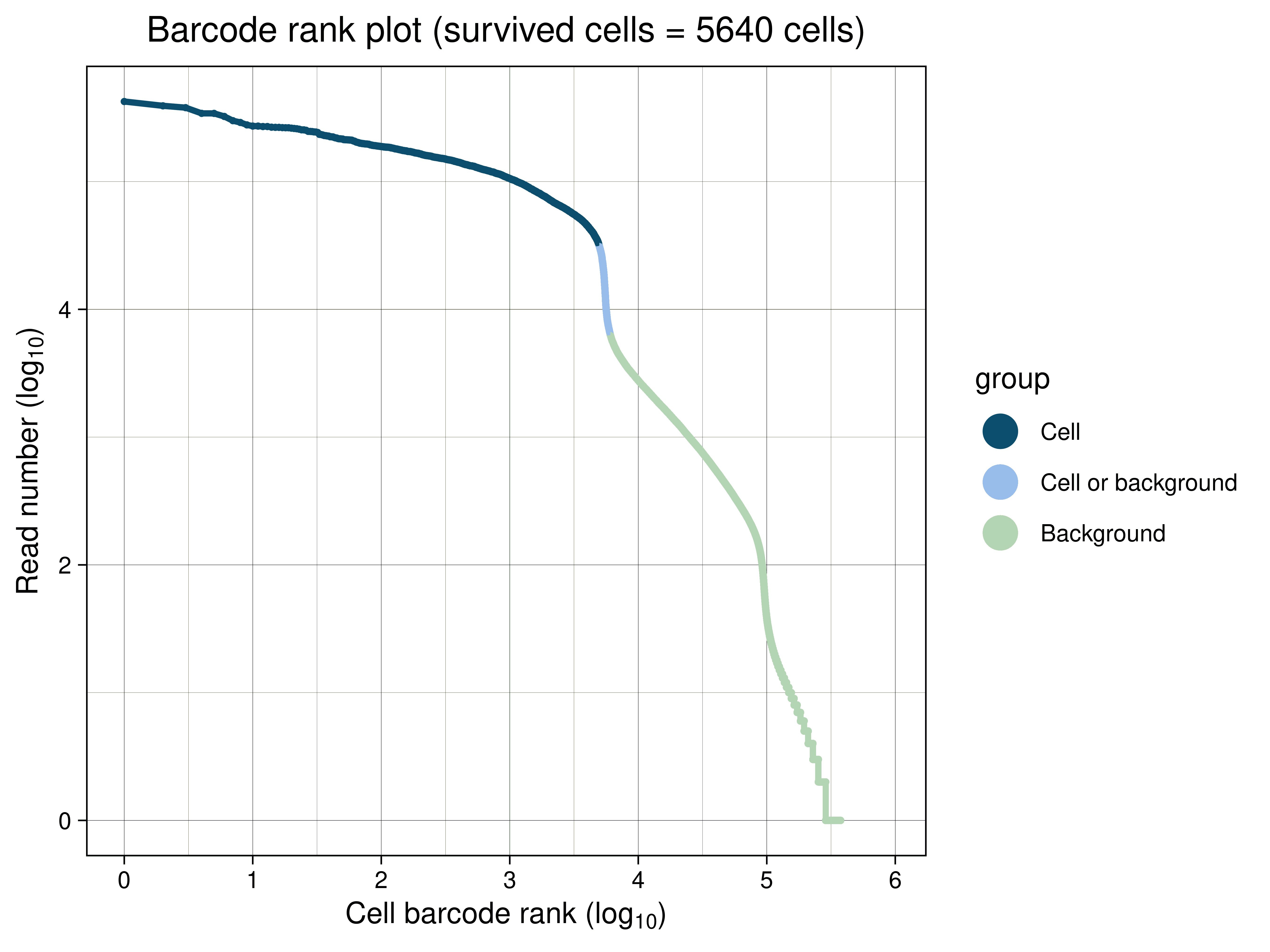
The vertical axis is the number of reads per cell barcode. The horizontal axis is the rank assigned to each cell barcode in order of number of reads per cell barcode. Inflection points are indicated by magenta vertical lines.
1) Data preprocessing
・
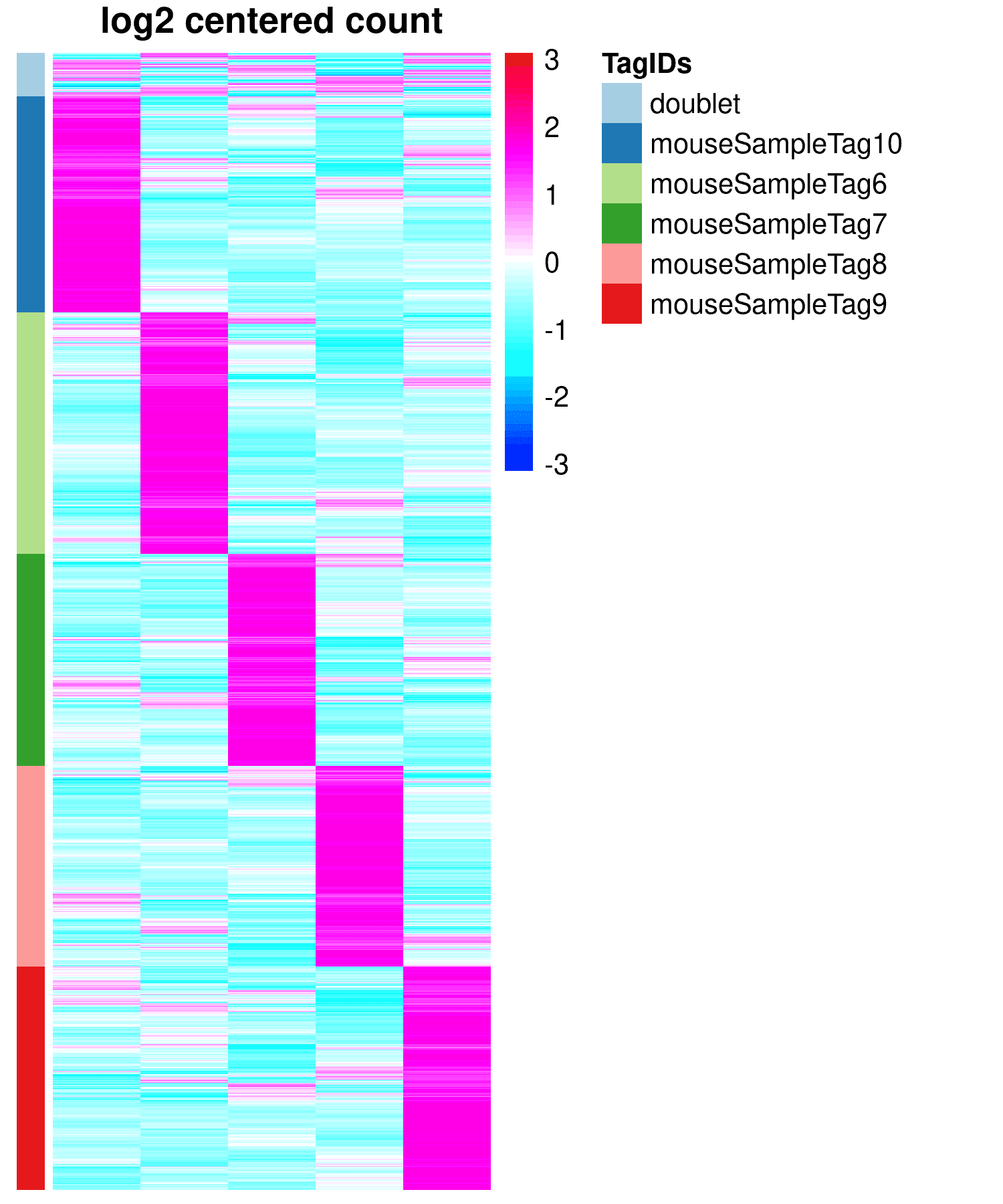
When multiple samples are analyzed simultaneously using tags (BioLegend's Hashtag, BD's Sampletag, etc.), the amount of tag expression in each cell is determined, and based on the amount of tag expression in each cell Determine which cells are from which samples (Fig.2, Table2)
Table 2 Number of cells assigned to each sample tag
図2
Fig.2 Heatmap showing the relationship between sample tag expression in each cell barcode and the TAG assigned to each cell Fig.
2) Pretreatment in Seurat
・
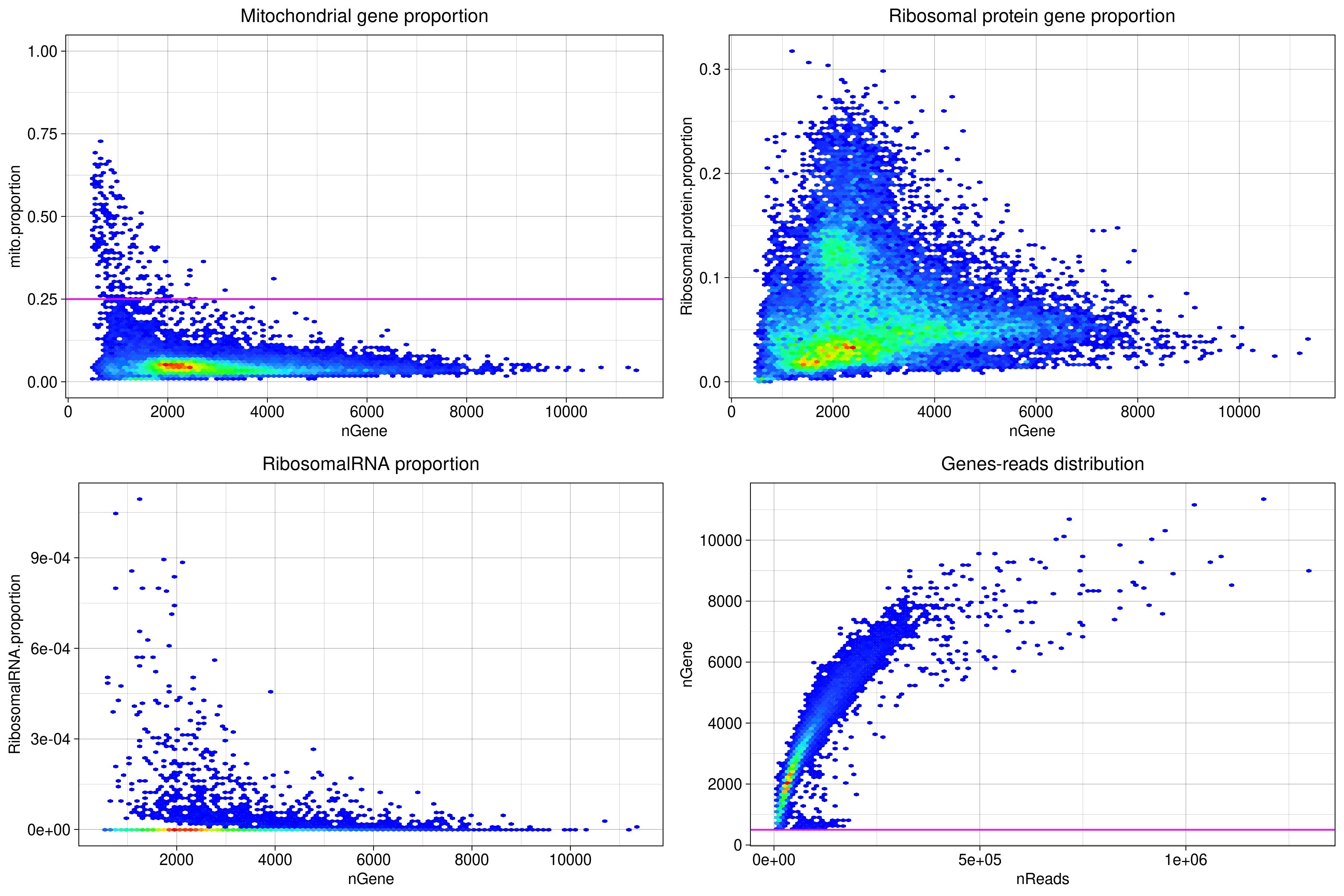
Removal of cells with high mitochondrial gene expression (>0.25) (Fig.3)
・
Remove doublet cells and cells that did not express the tag (for analysis using tag)
・
Scaling using the ScaleData function
・
Pseudocolor density plots and Ridgeplots are used to determine the number of genes detected and the distribution of expression numbers per gene to generally confirm that there are no problems.
Fig.3 Pseudocolor density plots of statistical data
In this Fig., one point corresponds to one cell, and where the cells overlap at the same location, the density of the overlap is determined, corresponding to a blue to red spectrum from the lowest density to the highest density, and The cells are represented by colors in the spectrum corresponding to their density.
3) Principal component analysis and JackStraw plots
After the FindVariableFeatures function is used to detect genes with large expression variation, a Principal Component Analysis (PCA) is performed on these genes. The number of principal components (PCs) used for clustering cells based on gene expression patterns is determined by Jackstraw analysis
Fig.4 JackStraw plot
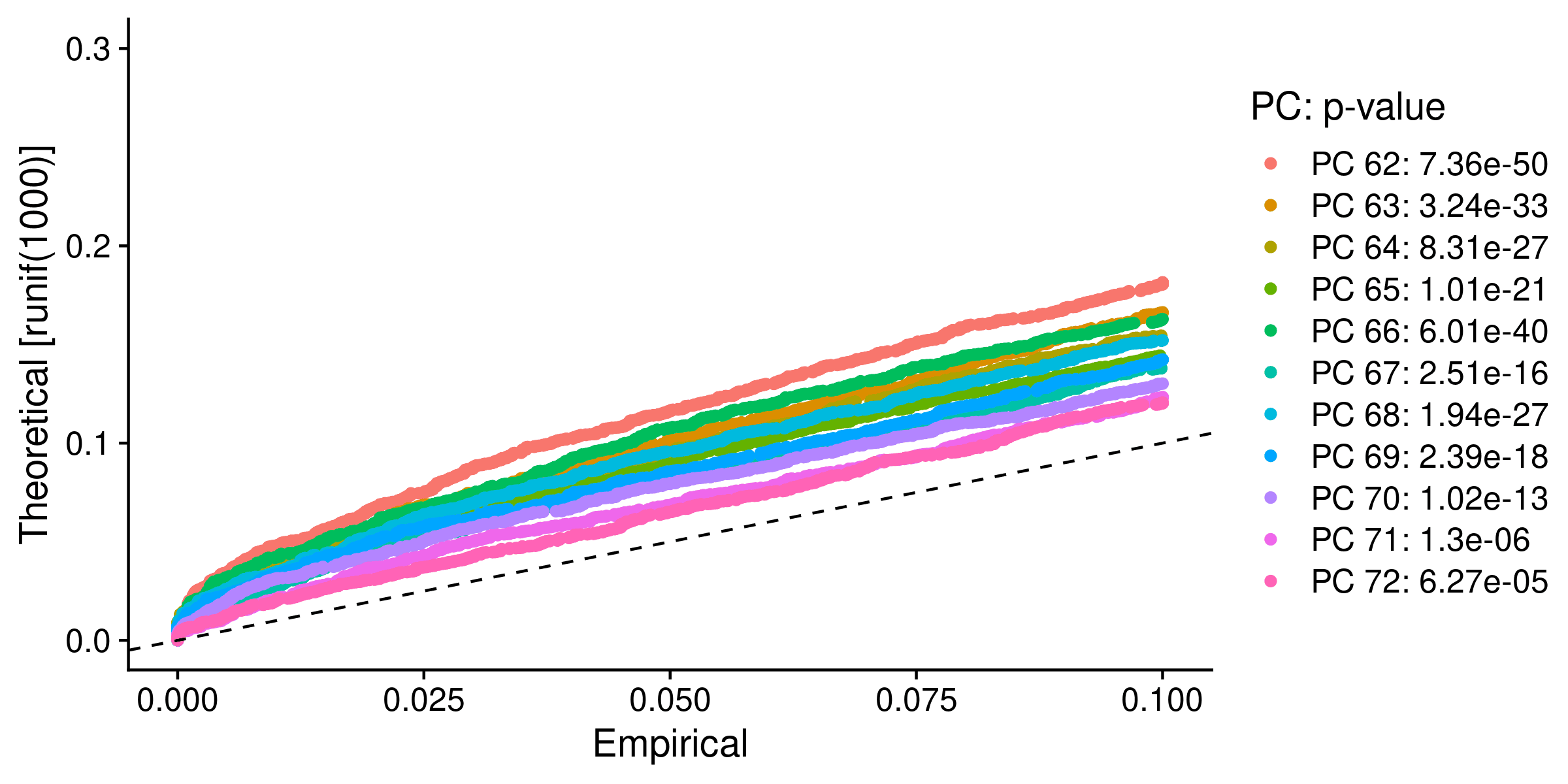
The number of principal components up to 71 with p-values less than 1 x 10⁻⁵ will be used in subsequent analyses.
4) Clustering
Perform cell clustering; cells with similar gene expression are in one cluster.
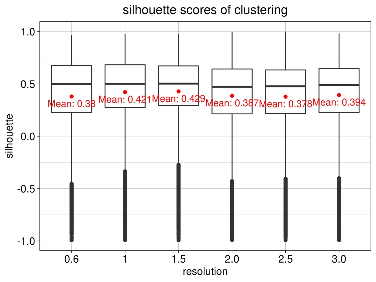
5) Seurat Clustering Silhouette Score Plot
Determine the resolution parameter. ( Fig.5) Here, the average silhouette score is maximum at resolution 1.5, so we assume that 1.5 is appropriate and proceed to the subsequent analysis.
Fig.5 Average silhouette score of clustering for each resolution parameter
6) Visualization of Seurat clustering results with Fit-SNE and UMAP plots
Visualize the clustering results done in 4) using FIt-SNE (George C. Linderman et al.Nat Methods 2019) (Fig.6) Also visualize with UMAP analysis (Fig.7)
Fig.6 Display of clustering results by Flt-SNE
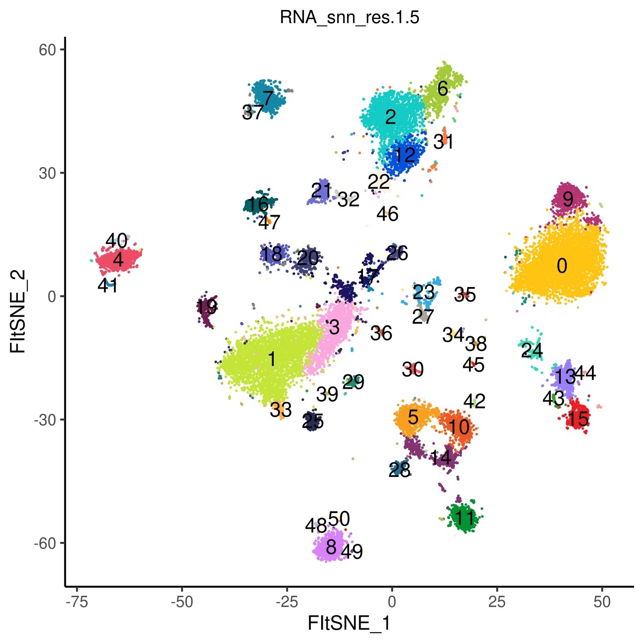
50 clusters were detected.
Fig.7 Display of clustering results by UMAP
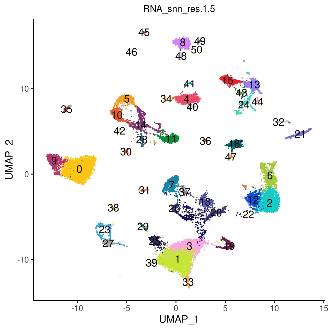
50 clusters were detected.
7) Analysis of cell composition in each sample
・
Find the number of cells in each cluster (Table 3)
・
Find differences in cell composition between samples (Fig.8, Fig.9)
Table 3: Number of cells in each cluster per tag (per sample)
0
529
785
558
526
587
1
672
640
458
352
651
2
284
272
334
273
338
3
228
243
198
172
208
4
182
150
167
135
176
5
114
232
164
138
120
6
171
130
150
158
149
7
167
148
100
213
113
8
113
210
159
110
123
9
121
146
140
110
157
・
Cluster numbers correspond to Suerat cluster numbers in Fig.6, Fig.7. Only 0 through 9 are shown in Table.
・
The original data is stored in .txt, or you can view the whole thing in an html file at Table.
図8
Percentage of total cells in each cell cluster is shown as a stacked bar graph for each sample Fig.
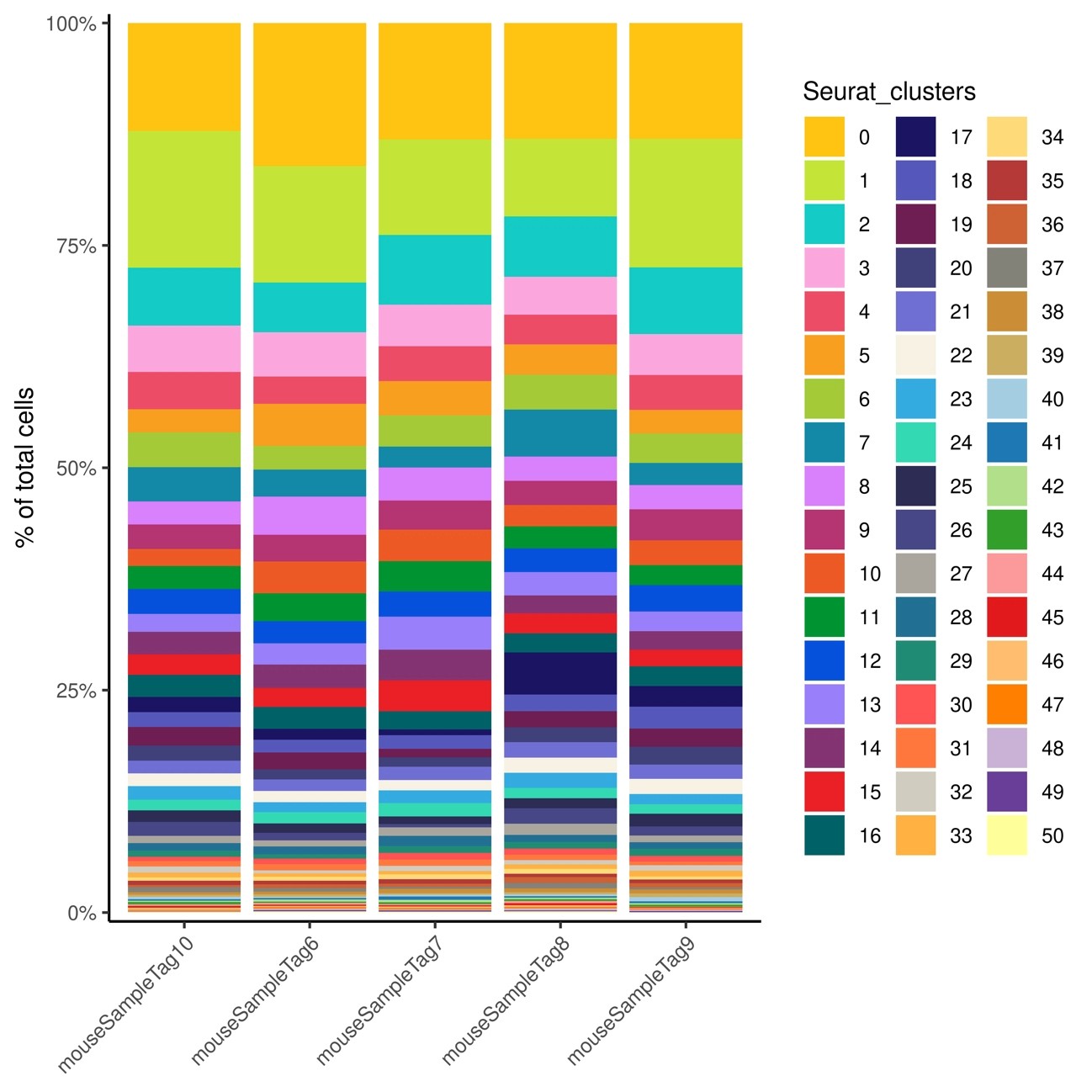
50 clusters were detected.
図9
Phylogenetic tree analysis of differences in cell composition percentages among samples
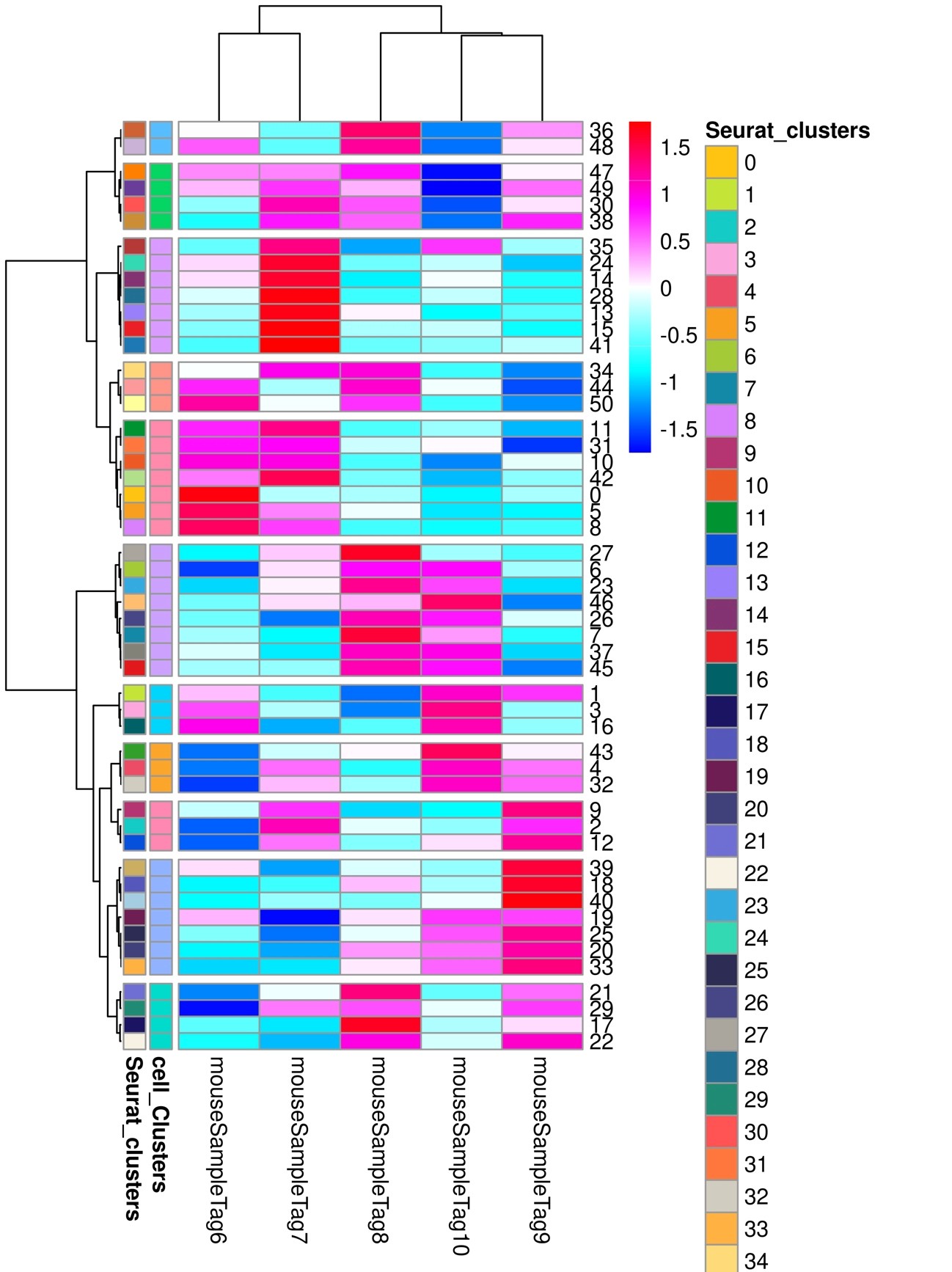
50 clusters were detected.
8) Detection of marker genes in each cell cluster
・
Find marker genes that are characteristically highly expressed in each cell cluster (Fig.10, Table4)
・
Expression patterns of the top 6 marker genes were visualized by FIt-SNE and UMAP (Fig.11, Fig.12)
Fig.10 Heatmap of expression patterns of the top 20 marker genes in each cluster Fig.
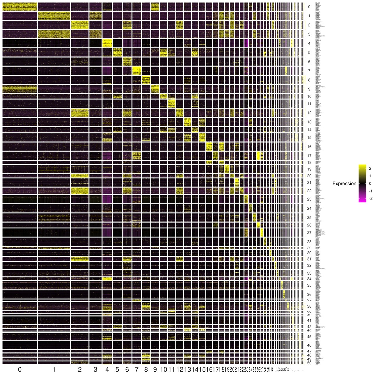
The vertical axis shows the 20 genes that are characteristic of each cluster, the horizontal axis shows the individual cells in each cluster, and the gene expression levels in the individual cells are indicated by the color of the spectrum on the right Table. The results can be used to determine the similarity of gene expression in individual cells within a cluster, or to compare gene expression in different clusters.
Table 4: All marker genes detected in each cluster
gene: Marker gene in a cluster
cluster: Seurat cluster
p_val_adj: bonferroni corrected p-value in the results of the variant gene test
logFC: change in log2 units of average expression in one cluster and all other clusters as Table
within_avg_exp: Average expression in a cluster (ln)
without_avg_exp: Average expression in all clusters except one (ln)
pct.1: Percentage of cells expressed in a cluster
pct.2: Percentage of cells expressed in all but the relevant cluster
p_val: p-value of the result of the variant gene test
*Marker gene tables are saved in .txt, and html files can also be used to search for gene and cluster names and sort the values.
Fig.11 Expression patterns of the top 6 marker genes in each cluster (Flt-SNE)
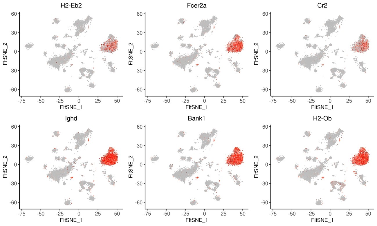
The html file can be toggled to show Tablefor each of the clusters shown in Fig.6.
Fig.12 Expression patterns of the top 6 marker genes in each cluster (UMAP)
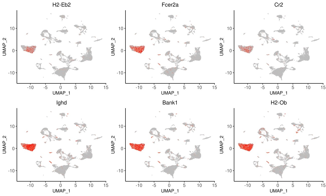
Among the clusters shown in Fig.7, the expression levels of each gene for cluster 0 are shown. The html file allows you to switch the display for each cluster.
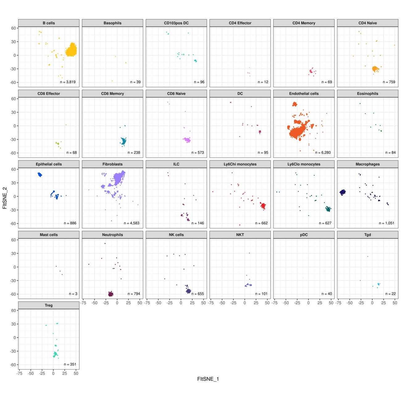
9) Estimation of cell types (Reference data)
The individual cell types in each cluster are estimated using the SingleR package (Fig.13, Fig.14). We recommend that you manually annotate and confirm what cells are in each cluster.
Fig.13 Percentage of estimated cell types in each cluster
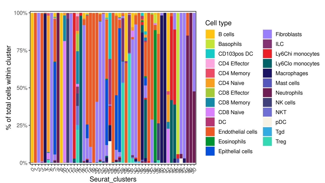
Fig.14 Display the distribution of each inferred cell type on FIt-SNE space

If you would like to request an analysis, please fill out and submit the hearing form at
We will prepare a quotation based on the information you send us.
TAS-Seq is a robust and sensitive amplification method for bead-based scRNA-seq
Human iPS cell-derived cartilaginous tissue spatially and functionally replaces nucleus pulposus
Combining an Alarmin HMGN1 Peptide with PD-L1 Blockade Results in Robust Antitumor Effects with a Concomitant Increase of Stem-Like/Progenitor Exhausted CD8+ T Cells
AMPK activation reverts mouse epiblast stem cells to naive state
Single cell transcriptomics clarifies the basophil differentiation trajectory and identifies pre-basophils upstream of mature basophils
Angiopoietin-like 4 is a critical regulator of fibroblasts during pulmonary fibrosis development
The early neutrophil-committed progenitors aberrantly differentiate into immunoregulatory monocytes during emergency myelopoiesis